Just machine learning

In this blog post, we’re going to talk about machine learning and its different types.

Artificial intelligence (AI) refers to machines that are programmed to learn and perform tasks that usually require human thinking, like recognizing images, understanding speech, making decisions, and translating languages.

Machine learning is a branch of AI that allows computers to learn and make predictions or decisions based on data. It uses algorithms and statistical models to analyze data, find patterns, and make predictions on new data.

Supervised Learning

Supervised learning is a machine learning technique where a model is trained on labeled data. The model is presented with inputs and corresponding outputs, and it learns to make predictions based on those inputs.

This technique is used for tasks such as classification, regression, and prediction.

Some common types of supervised learning include:

• Classification: the model learns to classify inputs into different categories or classes.
• Regression: the model learns to predict a continuous output based on the input.
• Time Series Prediction: the model learns to make predictions based on time series data.
• Anomaly Detection: the model learns to identify unusual or unexpected data points.

Classification

Classification is a type of supervised learning in machine learning where the model learns to put inputs into different categories or classes.

Examples → Image recognition, sentiment analysis, and speech recognition.

There are a bunch of algorithms that can be used for classification, including decision trees, random forests, and support vector machines (SVMs).

The choice of algorithm depends on the specific problem and the characteristics of the data. For example, decision trees are great for problems with just a few features, while SVMs are awesome when there are lots of features and the data isn’t linearly separable.

There are many algorithms that can be used for classification, including:

• Decision trees
• Random forests (Ensemble method)
• Support vector machines (SVMs)
• Nearest neighbor
• K-nearest neighbors (KNN)
• Naive Bayes

Let’s Discuss some of these techniques:

Decision Trees

Decision trees are a type of classification algorithm used in machine learning. They are especially handy for problems with just a few features and a ton of training examples.

The basic idea behind decision trees is to split up the input space into different regions, where each region represents a different class or category. This is done by recursively splitting up the input space over and over again based on the values of the input features.

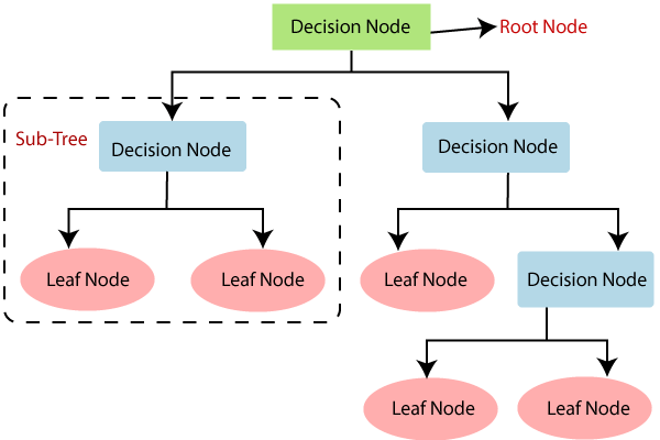
Fig: Decision Tree javatpoint

At each level of the tree, the algorithm picks the input feature that separates the training examples into different classes the best. This feature is used to make a decision node, which splits the input space into two or more regions. The process is repeated on each of the resulting regions until a stopping criterion is met, like reaching the maximum depth or having a minimum number of examples in each region.

Decision trees are super easy to understand and interpret, and they can be used for both classifying and regression problems. They can also handle non-linear relationships between the input features and the target variable.

from sklearn.tree import DecisionTreeClassifier
from sklearn.model_selection import cross_val_score

model = DecisionTreeClassifier(random_state=0)
model.fit(X_train, Y_train)

score = cross_val_score(model, X, Y, cv=10)

Decision trees can also be used for regression problems, where the goal is to predict a continuous output variable based on the input features. The decision tree algorithm works in the same way as for classification problems, but instead of predicting a class label, it predicts a numeric value.

Here is an example of a decision tree for a regression problem:

Regression Decision Tree

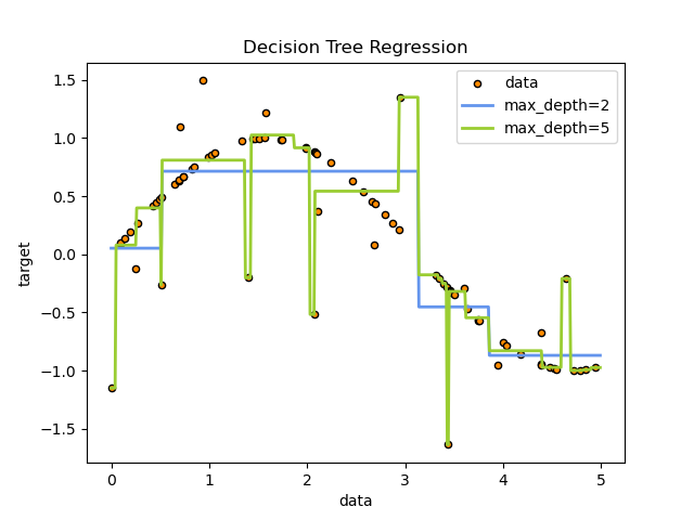
Fig: Regression Decision Tree scikit-learn

In this example, the decision tree is used to fit a sine curve as a result it learns linear regression approximating the sine curve. We can see in this example, that if max depth of the tree is set to high, it can overfit the training data by learning the noise observations also.

The algorithm chooses the feature that results in the best split of the data based on a measure of the variance reduction. The prediction for each leaf node is the average of the target values of the training examples that fall within that leaf node.

However, decision trees can be sensitive to small changes in the input data and may overfit the training data if not properly regularized. To address these issues, ensemble methods such as random forests and gradient boosting are often used.

Overall, decision trees are a simple and effective technique for classification and regression problems, particularly when the decision boundary is simple or linear.

Nearest-neighbor classification

In this algorithm, the model given an input chooses the class of the nearest data point to that point.

This technique is useful for problems where the decision boundary between classes is complex or nonlinear. However, it can be computationally expensive and may not perform well on high-dimensional data.

K-Nearest Neighbor Classification (KNN)

In this algorithm, the model assigns a class to a new data point based on the classes of the k nearest data points in the training data set. The value of k is a hyperparameter that can be tuned to optimize the model’s performance.

This technique is often used for problems with a small number of classes and a large number of features. However, it can be sensitive to the choice of distance metric used to calculate the distance between data points.

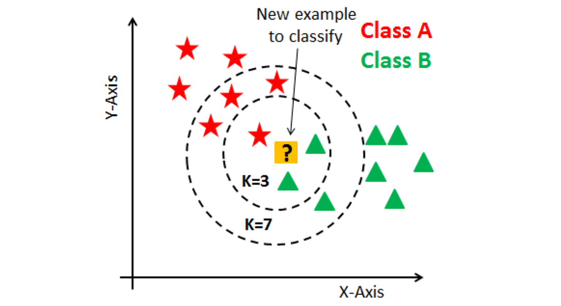
Fig: KNN Example medium

Overall, k-nearest neighbor classification is a simple and effective technique for classification problems, particularly when the decision boundary is complex or nonlinear.

Regression

Regression is a type of supervised learning in machine learning. It involves the use of algorithms and statistical models to predict a continuous output based on input data.

This is useful when trying to predict a value that falls within a range, such as the price of a house based on its size, location, and other factors.

Example → f(size, location, architecture) = price f(1200, Delhi, 2 story building) = 1 million

Types of Regression

There are several types of regression, including:

• Linear Regression: the model learns to predict a continuous output based on a linear relationship between the input and output variables.

  

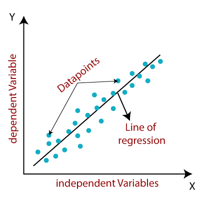
    # using skitit learn
    from sklearn.linear_model import Linear Regression
      
    model = LinearRegression()
    model.fit(X_train, Y_train)
      
    # Print coefficients and accuracy
    print(model.coef_)
      
    accuracy = model.score(X_test, Y_test)
    print(accuracy)
  

• Logistic Regression: the model learns to predict a binary output based on the input variables.
• Polynomial Regression: the model learns to predict a continuous output based on a polynomial relationship between the input and output variables.
• Ridge Regression: a regularization technique used to prevent overfitting in linear regression models.
• Lasso Regression: a regularization technique used to prevent overfitting in linear regression models, but with a different approach than Ridge Regression.
• Elastic Net Regression: a combination of Ridge and Lasso Regression, which balances their strengths and weaknesses.

Each type of regression is suited for different types of data and problems, and choosing the right type of regression is an important part of building an accurate machine learning model.

Logistic Regression

Logistic regression is a type of supervised learning in machine learning that is used for binary classification tasks. In this technique, the model learns to predict a binary output (0 or 1) based on the input variables.

It is commonly used in applications such as fraud detection, spam filtering, and medical diagnosis.

The logistic regression algorithm uses a sigmoid function to map the input values to a range between 0 and 1 (generate probabilities), which represents the probability of the input data belonging to one of the two categories. The algorithm then makes a binary decision based on this probability.

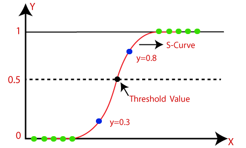
Fig: Logistic regression javatpoint

# Logistic Regression
from sklearn.linear_model import LogisticRegression
from sklearn.metrics import accuracy_score

model = LogisticRegression()
model.fit(X_train, Y_train)

accuracy = accuracy_score(model.predict(X_test), Y_test))
print(accuracy)

Ridge Regression

Ridge regression is a type of linear regression that adds a regularization term (L2) to the cost function to prevent overfitting. The cost function for ridge regression is:

The Ridge Regression Equation is given by:

$J(w) = \sum_{i=1}^{m} [y^{(i)} - \hat{y}^{(i)}]^2 + \alpha\sum_{j=1}^{n} w_j^2$

where:

• J(w) is the cost function
• m is the number of training examples
• n is the number of features
• y is the target variable
• w is the vector of coefficients
• α is the regularization parameter

The first term in the equation is the mean squared error (MSE) between the predicted values and the true values. The second term is the L2 regularization term, which penalizes the magnitude of the coefficients.

Lasso Regression

Lasso regression is another type of linear regression that adds a regularization term (L1) to the cost function. The cost function for lasso regression is:

$J(w) = \sum_{i=1}^{m} [y^{(i)} - \hat{y}^{(i)}]^2 + \alpha\sum_{j=1}^{n} \lvert w_j \rvert$

Where:

• $J(w)$ is the cost function
• $m$ is the number of training examples
• $n$ is the number of features
• $y$ is the target variable
• $w$ is the vector of coefficients
• $\alpha$ is the regularization parameter (hyperparameter)

The first term in the equation is the mean squared error (MSE) between the predicted values and the true values. The second term is the L1 regularization term, which penalizes the absolute value of the coefficients.

Lasso regression is useful for feature selection, as it tends to set the coefficients of less important features to zero. This can lead to a more interpretable model and improve its generalization performance.

Unsupervised Learning

Unsupervised learning is a type of machine learning where the model is trained on unlabeled data. The model is not given any specific outputs to learn from, but instead must identify patterns and relationships in the input data on its own.

This technique is used for tasks such as clustering, anomaly detection, and dimensionality reduction.

Some common types of unsupervised learning include:

• Clustering: the model learns to group similar inputs into clusters or categories.

  But how you do clustering?

• Anomaly Detection: the model learns to identify unusual or unexpected data points.
• Dimensionality Reduction: the model learns to identify the most important features or variables in the input data.
• Density estimation involves a model learning a probability density function (PDF), which is used in anomaly detection. Instances found in very-low density regions are considered anomalies.

Unsupervised learning is useful when working with large amounts of data that may not be well understood or labeled. By identifying patterns and relationships in the data, unsupervised learning can help to uncover insights and guide further analysis.

Reinforcement learning

Reinforcement learning is like a cool type of machine learning where an agent learns to make decisions based on a reward system. The agent gets to interact with an environment, taking actions and getting feedback in the form of rewards or penalties. Over time, the agent gets smarter and learns to make decisions that give it the most rewards.

This technique is used for things like game playing, robotics, and autonomous driving. It’s all about teaching machines to make complex decisions and do cool things in the real world.

Reinforcement learning is really powerful and has lots of cool applications, but it can also be kind of complex and take up a lot of computer power. So, before you decide to use reinforcement learning, you should think about the problem and the data you have.

Ensemble Methods

A group of predictors is called ensemble and an ensemble learning algorithm is called Ensemble method.

In other words, Ensemble methods are a type of machine learning technique that involve combining multiple models to improve their performance.

Ensemble has a similar bias but a lower variance than a single predictor trained on a the original training set.

There are several types of ensemble methods (algorithms), including:

Bagging

The model combines the predictions of multiple models trained on different subsets of the training data. This can help to reduce overfitting and improve the accuracy of the model.

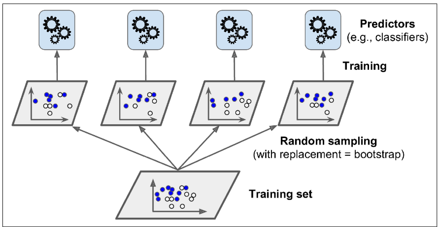
Fig: Bagging and pasting involves training several predictors on different random samples of the training set

Bagging - sampling is performed with replacement (bootstrap=True)

Pasting - sampling is performed without replacement (bootstrap=False)

from sklearn.ensemble import BaggingClassifier
from sklearn.tree import DecisionTreeClassifier

bag_clf = BaggingClassifier(
    DecisionTreeClassifier(), n_estimators=500,
    max_samples=100, bootstrap=True, n_jobs=-1
)
bag_clf.fit(X_train, y_train)

y_pred = bag_clf.predict(X_val)
print(y_pred)

n_estimators = number of decision trees

max_samples = 100 training samples randomly sampled from training set

bootstrap = True, with replacement

n_jobs = number of CPU cores to use for training and predictions, -1 means use all available

Bootstrapping introduces more diversity into the predictor, means it is more biased than pasting; but the diversity also means the predictors are less correlated and ensemble variance is reduced.

Random Forests

Random Forest is an ensemble of Decision trees, generally trained via the bagging method (or sometimes pasting), typically with max_samples set to the size of training set.

from sklearn.ensemble import RandomForestClassifier

rnd_clf = RandomForestClassifier(n_estimators=500, max_leaf_nodes=16, n_jobs=-1)
rnd_clf.fit(X_train, y_train)

y_pred_rf = rnd_clf.predict(X_val)

Random Forest algorithm introduces extra randomness when growing trees; instead of searching for the best feature when splitting a node, it searches for the best feature among a random subset of features.

Feature Importance

Random forests allow us to measure the relative importance of each feature. Feature importance is calculated by how much tree nodes that use that use that feature reduce impurity on average.

# feature importance
for name, score in zip(iris["feature_names"], rnd_clf.feature_importances_):
    print(name, score)

# output
# sepal length (cm) 0.10109300798027078
# sepal width (cm) 0.031280365249363895
# petal length (cm) 0.3941268382545283
# petal width (cm) 0.47349978851583696

Random forests are particularly useful for high-dimensional data and problems with complex decision boundaries. They can also handle missing values and noisy data.

Overall, random forests are a powerful and versatile technique for solving a wide range of machine learning problems.

Boosting

The model combines the predictions of multiple weak models to create a strong model. This can help to improve the accuracy of the model and reduce bias.

AdaBoost

A type of boosting ensemble method used for classification problems. AdaBoost combines the predictions of multiple weak models using a weighted sum, where the relative weight of misclassified instances increased (boost).

The algorithm increases the relative weight of the misclassified training instances.

from sklearn.ensemble import AdaBoostClassifier

ada_clf = AdaBoostClassifier(
    DecisionTreeClassifier(max_depth=1), n_estimators=200, 
    algorithm="SAMME.R", learning_rate=0.5
)
ada_clf.fit(X_train, y_train)

Gradient Boosting

A type of boosting ensemble method used for classification and regression problems. Gradient boosting tries to fit the new predictor to the residual errors (literally) made by the previous predictor.

The basic idea behind gradient boosting is to build a sequence of models, each of which tries to correct the errors of the previous models. The final prediction is the weighted sum of the predictions of all the models in the sequence.

For example, in a binary classification problem, the first model might predict the probability of the positive class for each example. The second model would then focus on the examples that were misclassified by the first model, and try to improve the predictions for those examples. The third model would then focus on the examples that were still misclassified by the first two models, and so on.

from sklearn.ensemble import GradientBoostingClassifier

model = GradientBoostingClassifier(n_estimators=1000, learning_rate=0.5, max_depth=1, random_state=0)
model.fit(X_train, Y_train)

score = model.score(X_test, Y_test)
print(score)

Gradient boosting with early stopping:

import xgboost

xgb_reg = xgboost.XGBRegressor()
xgb_reg.fit(X_train, y_train)

xgb_reg.fit(X_train, y_train,
           eval_set=[(X_val, y_val)], early_stopping_rounds=2
           )

y_pred = xgb_reg.predict(X_val)

Gradient boosting is a powerful technique for improving the performance of machine learning models, particularly when working with complex data or when the performance of a single model is not sufficient. However, it can be computationally intensive and may require careful tuning of hyperparameters to achieve good performance.

Stacking

The model combines the predictions of multiple models using a meta-model (blender). This can help to improve the accuracy of the model and reduce overfitting.

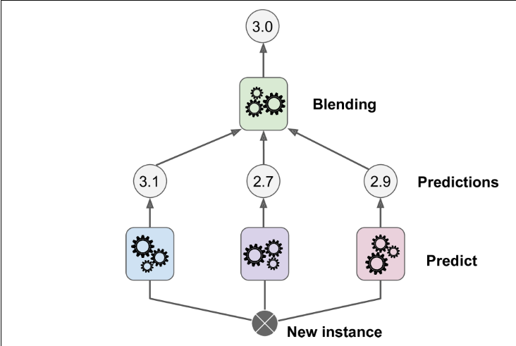
Fig: Aggregating predictions using a blending predictor

Ensemble methods are particularly useful when working with complex data or when the performance of a single model is not sufficient. By combining the predictions of multiple models, ensemble methods can help to improve the accuracy and reliability of the model.

Overall, ensemble methods are a powerful technique for improving the performance of machine learning models, and they are widely used in industry and research. However, it is important to carefully consider the problem and the available data before choosing an ensemble method.

References

Kaggle Notebook

Hands on Machine Learning - buy